Runge-Kutta method vs Euler method

In this post, I will compare and contrast two of the most well known techniques for the solving of systems of differential equations. The Runge-Kutta method is named for its’ creators Carl Runge(1856-1927) and Wilhelm Kutta (1867-1944). The Runge-Kutta method is very similar to Euler’s method except that the Runge-Kutta method employs the use of parabolas (2nd order) and quartic curves (4th order) to achieve the approximations. In essence, the Runge-Kutta method can be seen as multiple applications of Euler’s method at intermediate values, namely between and . I will be focusing on the 4th order method, as it is the most common method for obtaining graphical representations of systems of equations. Any referrals to the “RK method” are in reference to the Runge-Kutta 4th order method for solving systems of differential equations.

The backbone of the RK method lies in the idea of using a weighted average of the slopes of field segments at four(4) points very close to the current point, , of whom’s location is determined by applying Euler’s method. If we assume that we know the location , which is the Euler approximation of the function . To obtain the next approximate solution, , we must apply the fundamental theorem of calculus (developed by Sir Isaac Newton and/or Gottfried Wilhelm Leibniz, this argument is a complete topic of it’s own). The theorem says:  = . In order to obtain an approximation of this integral, Simpson’s rule must be applied. Simpson’s rule states: .

Now, the RK method’s backbone lies in the use of a “weighted average” of the slopes at four points near our current point. To obtain the fourth point, two evaluations must be made the the middle point, . The approximation then becomes . To begin calculating the approximation, we must start the first of our four evaluations. Doing this requires us to calculate the slope of the line that passes through our initial point . In order to find this slope, the value of the function must be computed. As is common with most demonstrations of the RK method, label this slope k1.

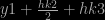
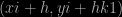
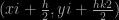
Here is where the first real difference between the RK method and the Euler method arises. The next step in the Euler method tells us that the next value will be while the RK method takes half of this increase in the y coordinate, , and goes halfway between the original and the next step .

The next step is to perform the second evaluation.  The x value of our point is and the y value is . In order to calculate the slope at this point, we must evaluate the function at the point . The value of this slope is to be labeled k2.

The Euler method would have us move one step size to the point 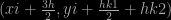. Just as in the last step, with the RK method, we take half of this increase leaving us at the point . As is required with the RK method, we must calculate the slope at this by evaluating the function . The value of this slope is to be labeled as k3. If we move along this slope for one step size, we would be at the x value and the y value . The y value differs only from the last value by . We now move to the x value and the y value which accounts for the last increase.

The final evaluation is to be made at this point by calculating the slope of the solution which passes through the point . This slope is to be labeled  k4. This value is not the original value predicted by Euler’s method. After performing these evaluations, we now have four slopes very close to the point ; one at , one at and two at . In order to determine the next point, the RK method takes a weighted average of these slopes.

.

As is similar with the Euler method, it is possible to put a bound on the error between the exact solution value, 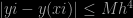and the approximate value calculated with the RK method. This difference  is the  local truncation error; , where M is a constant depending on the function and the specified interval.

So why go through all this extra work when the Euler method seems much quicker and to the point? The fact is, the Euler method provides a very shallow approach to the solutions that we desire from differential equations. In order to achieve a more accurate approximation with the Euler method, we must decrease the step size. By decreasing the step size, the amount of steps required to reach the desired point greatly increases, thus greatly increases the amount of meticulous calculations that must be done. While, on the other hand, the RK method may be a bit more complicated, the error is almost non existant after the first application of the method.

An interesting example of why the RK method is much, much more effective than the Euler method can be shown by examining some of the world’s most interesting curves, namely the Lorenz attractor and the Rossler attractor. The first curve I will examine is the Lorenz attractor. (Most of the following information is gathered from Jonas Bergman’s Doctoral thesis, titled  Knots in the Lorentz system ca 2004).

The Lorenz attractor was introduced by Edward Lorenz in 1963, and is a 3D structure that corresponds to the long term behavior of a chaotic flow. The attractor shows how the state of a dynamic system( the three variables of a three dimensional system) and how they evolve over time in a complex, non repeating pattern. The attractor itself, comes from simplified equations of convection rolls arising in the atmosphere.

The Lorenz equations are a set of three coupled non-linear ordinary differential equations. They make up a simplified system describing the two-dimensional flow of a fluid. As can be seen, the derivative of all three variables is given with respect to t, and as a function involving one or both of the other variables. The three equations are as follows:

The most common associated values associated with the graphical representation of the lorenz attractor are: sigma = 10, r= 28, and b = 8/3.

To obtain a graph of the Lorenz attractor I created an m file containing the following:

[T,Y]=threeplot(‘lorenz’,0.1,0.1,0.1,0,30);

function F=lorenz(t,vec)

sigma=10.0;
rho=28.0;
beta=2.66666666;

x=vec(1);
y=vec(2);
z=vec(3);

F(1)= sigma* (y -x);
F(2)= rho* x – y – x*z;
F(3)= -beta* z + x*y;

F=transpose(F);

Then I plotted it with matlab using the plot3 command and obtained the following:

As you can see, this is a truly remarkable system of equations. To see just how chaotic the values of x,y, and z change I will borrow a figure from the esteemed British Mathematician Lewis Dartnell, in which x=red, y=green, z=blue.

It is clearly evident that there exists no pattern in the behavior of this attractor. Numerical analysis of such behavior is very difficult. One of the properties of a chaotic system is that it is sensitive to initial conditions. This means that no matter how close two different initial states are, their trajectories will soon diverge. This property indicates that accuracy is pivotal in obtaining any sort of a reasonable solution. Methods such as Euler’s method will not provide even a close approximation. Why you may ask? Euler’s method gives us an approximation of a solution. This approximation is close to what the solution curve may look like in most cases, but in this case the error produced by the Euler will ultimately skew the results. Even decreasing the step size to an almost infintesimally small size will not provide a solution, as millions small steps along the slope would have to occur. This is popularly referred to as the “Butterfly Effect”, whereby small changes in the initial state can lead to rapid and dramatic differences in the outcome, especially in this case. Whereas the RK method provides us with a very reasonable solution to such systems. In the RK method, the lower order “error” terms will inevitably cancel out, providing a proper representation of the behavior of the Lorenz system.

Another chaotic system that displays the superior approximation of the RK method as opposed to the Euler method is the Rossler attractor. (Most of the information on the Rossler attractor is obtained from Rossler’s 1976 publication titled An Equation for Continuous Chaos). Otto Rossler published his paper on the Rossler attractor in 1976, intending for it to behave similarly  to the Lorenz attractor. The behavior of the attractor is best summarized by it’s creator in his original publication ” An orbit within the attractor follows an outward spiral close to the x,y plane around an unstable fixed point. Once the graph spirals out enough, a second fixed point influences the graph, causing a rise and twist in the z-dimension. In the time domain, it becomes apparent that although each variable is oscillating within a fixed range of values, the oscillations are chaotic”(Rossler 103).

The equations that define this chaotic system are:

.

Two sets of values are most commonly used to illustrate the behavior of this system, namely a=0.2, b=0.2, c=5.7, and a=0.1, b=0.1, and c=14. The latter of the two sets has been used to display the systems behavior in recent years.

To obtain a graph of the Rossler attractor, I created an m file in matlab. The code is as follows:

function F=Rossler(t,vec)
 a=0.2;
 b=0.2;
 c=5.7;
 x=vec(1);
 y=vec(2);
 z=vec(3);
 F(1)= -y-z;
 F(2)= x+a*y;
 F(3)= b+z*(x-c);
 F=transpose(F);

Plotting the results using the plot3 command yields

Again, the systems chaotic behavior is very evident.

The chaotic behavior of the Rossler system is readily evident from the behavior of the graph. Borrowing another time series from Lewis Dartnell, with x=red, y=green, and z=blue, the results are changing at such a chaotic rate that they are almost impossible to distinguish from one another.

With the behavior changing so rapidly, the room for error is next to nothing. Just as in the Lorenz system, the “approximation” obtained from the Euler method will not give us an acceptable answer. In order to obtain even a remotely accurate model with the Euler method, the step size would have to be infintesimally small, and would take an obscure amount of time to accomplish. While, with the RK method, all of the lower order “error” terms cancel out, yielding a reasonable approximation to the behavior of the system.

While both the RK method and the Euler method have strengths and weaknesses, in the analysis of dynamic time varying chaotic systems, the RK method towers over the almost obsolete Euler method. With the room for error being so small in such an erratic system, one is forced to use the most accurate of numerical approximation techniques, and in these cases, this is generally associated with the RK 4th order method.